Kinematics
Kinematics is a physics framework useful for solving problems involving position, velocity and acceleration of particles without regard to mass or the forces which caused acceleration.
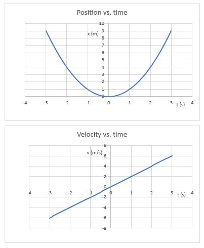
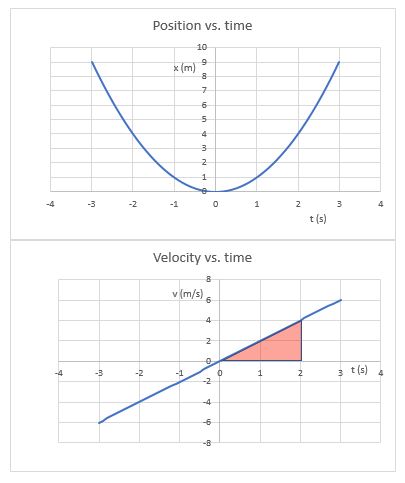
Position and velocity vs. time graphs
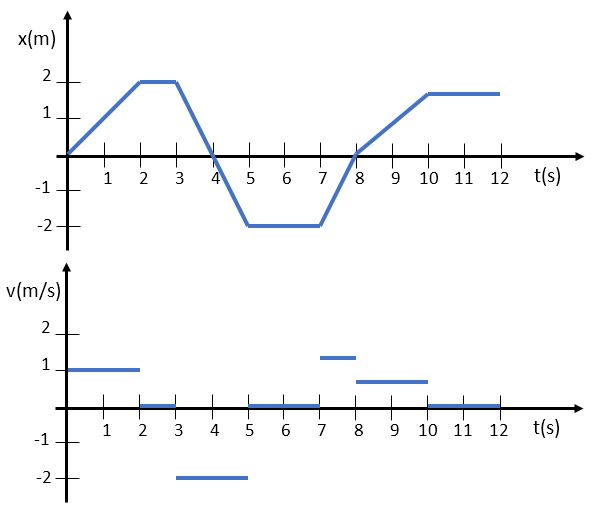
A velocity vs. time graph depicts the slope of the corresponding position vs. time graph. The motion in the above graph depicts an object moving with constant velocity during the time increments.
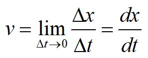
The object depicted in the graphs above does not have constant velocity. The instantaneous velocity at any point in time is given by the slope of a line tangent to the position graph at that time. The value of the instantaneous velocity is equal to the slope of the tangent line.
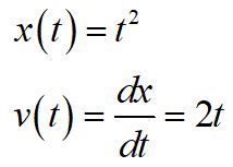
The function governing the motion of the particle is parabolic, so the velocity of the object is linear, since it is the time derivative of the position function.
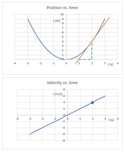
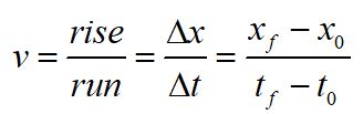
You can also see that the slope of the tangent line of the x vs. t curve gives the value of the v vs. t curve at the corresponding time. Here, the rise/run of the tangent line at t = 2 seconds is 4/1, and the corresponding velocity at that time is 4 m/s.
We can also do the inverse operation to find the change in position from the velocity graph. The integral of v vs. t gives the area under the curve, which is equal to the change in position during the corresponding time interval.
Here, the area under the curve equals half of the rectangle that is 4 m/s high and 2 s wide, so the A = (4 m/s)(2 s)/2 = 4 m.
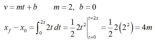
We get the same answer analytically by taking the integral of the velocity function over the time interval.
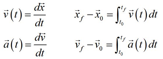
In general, velocity is the time derivative of position and acceleration is the time derivative of velocity. Position is the time integral of velocity and velocity is the time integral of acceleration.
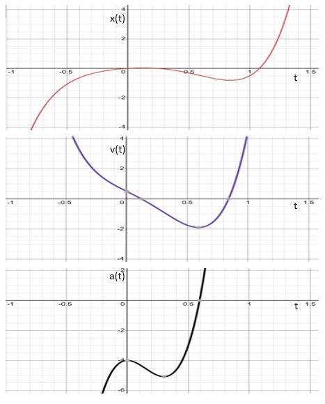
Graphs of generic position, velocity and acceleration functions illustrates that velocity is the slope of the position function and acceleration is the slope of the velocity function. For example, where the slope of the position function equals at a minimum or maximum, the value of the velocity function is zero.
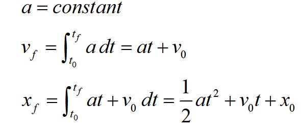
For constant acceleration, we get useful forms for solving problems involving position, velocity and acceleration. These equations are commonly called the "kinematic equations." Please keep in mind that they are only valid for constant acceleration.
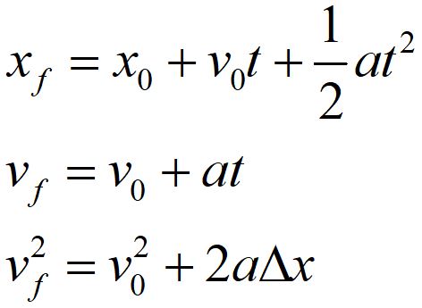
We typically write the kinematic equations for constant acceleration in the forms shown above.
Using substitution, we can consolidate the first two equations into the form shown in the third equation.
Practice problems:
1. Find the position vs. time and acceleration vs. time functions for the velocity vs. time function: v(t) = 3t2 - 8t3.
2. The position of a particle is given by x = 5t3 - 18t2. When is the particle's velocity at a minimum?
3. A particle starts from rest at the origin and moves according to the function v(t) = 3.2 A t2 - 2.2 B t.
How far is the particle from the origin at t = 1.6 s?
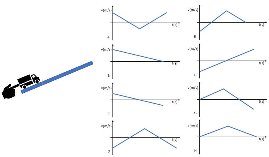
4. You give a toy truck a short push upward on a ramp, and it goes up the ramp a ways and then rolls back down.
Which plot could depict the velocity vs. time graph for the truck?
Just consider motion after you have stopped touching the truck. Assume the positive direction is defined as being up the ramp.